How to correctly use spectrum analyzers for EMC pre-compliance tests
November 26, 2021
In this note, we discuss EMC pre-compliance test parameters and how different settings affect your measurements. There are also sensitivity considerations and tips for the protection of the spectrum analyzer during tests.
Index
3. Standards-related requirements
4. Internal attenuator/pre-amplifier
6. General sensitivity considerations
6.1 Conducted noise testing with LISN
6.2 Conducted noise testing with RF current probes
6.3 Radiated noise testing with TEM-cells
6.4 Radiated noise testing with antennas
1. Introduction
A spectrum analyzer is a key instrument for conducting EMC testing. Analyzers with EMC-specific features have become very affordable in recent years and these are usually sold as “EMI-options” that typically include CISPR filters and Quasi-Peak (QP) detectors in addition to the standard features of spectrum analyzers.
Spectrum analyzers offer a wide range of parameter settings and need to be set up correctly in order to make measurements as close as possible to the requirements of the specific EMC standards that apply to the product’s design and end-use. EMC standard-related requirements determine the correct instrument settings of the RBW filter, video bandwidth (VBW), detector type, frequency span, and sweep time. Radiation limits and transducer characteristics also affect the required settings. Optimizing the instrument is necessary to achieve a good compromise between high sensitivity and low distortion.
Measurement plots documented in this application note are created using a Siglent SSA3021X Plus, an entry-level EMI- spectrum analyzer with an excellent price-performance ratio.
2. Relevant standards
Several standards specify EMC test setups and requirements for measurement equipment. Most prominent are the CISPR 16 and EN 61000-4 series. There are additional relevant standards, such as CISPR 25, Mil-461, DO 160, and more. This document is mainly focused on the CISPR 16 standard to keep this application note as compact as possible.
3. Standard related requirements
3.1 Amplitude units
In RF applications, [dBm] is the predominant amplitude unit. [dBm] is a logarithmic power unit, which makes sense, as input and output impedance of RF building blocks are typically designed to 50 Ohm.
In EMC pre-compliance applications, the impedance of EUTs and power supply sources is hardly predictable. Consequently, emission limits are predominantly specified in [dBµV] and [dBµA] amplitude units. Standardized transducers such as Line Impedance Stabilized Networks (LISNs), Coupling/Decoupling Networks (CDNs), RF current probes, and others are used to establish interfaces with defined impedance, in order to connect 50 Ohm measurement equipment.
3.2 Resolution bandwidth
Typically, the resolution bandwidth filters on spectrum analyzers use Gaussian shaped Intermediate Frequency (IF) filters with adjustable bandwidths that follow a 1 -3 -10 sequence, e.g. 100 Hz, 300Hz, 1 kHz, 3kHz, 10 kHz, 30 kHz…
In order to be compliant with CISPR standards, the spectrum analyzer must additionally provide so-called CISPR-filters. Many analyzers use a Gaussian filter by default, so the user should select the EMI filter option if required.
In Figure 1 below, there is a comparison between the Gaussian and CISPR filter shapes:
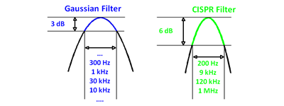 Figure 1: Gaussian and CISPR filter shapes.
Besides specifying filter shape, impulse response, and sidelobe suppression, CISPR specifies frequency bands and the corresponding filter bandwidths that have to be used:
| Frequency range | CISPR filter bandwidth |
| 9 kHz – 150 kHz | 200 Hz |
| 150 kHz – 30 MHz | 9 kHz |
| 30 MHz – 1 GHz | 120 kHz |
| Above 1 GHz | 1 MHz |
Table 1: CISPR frequency range and filter bandwidth setting.
The smaller the resolution bandwidth (RBW), the lower the base noise level. The base noise level is a function of the measurement instruments Displayed Average Noise Level (DANL), the measurement transducer/antenna/probe, and the environmental RF present during the measurement. You may already have observed steps in test house plots, which are caused by switching filter bandwidth. Figure 2 below shows an example of such a step where the RBW was changed from 9 kHz in the first part of the sweep to 120 kHz after 12 MHz:
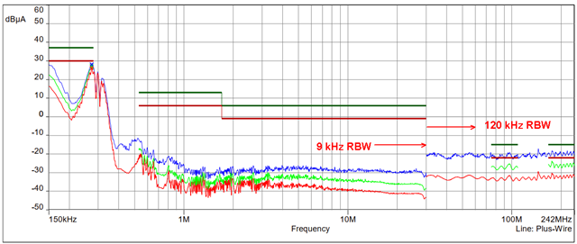
Figure 2: Transition from 9 kHz to 120 kHz RBW at 30 MHz – Note steps in the base noise level.
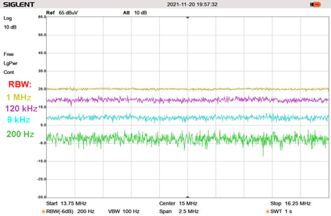
Figure 3: Spectrum analyzer DANL level versus resolution bandwidth.
3.3 Frequency resolution
Spectrum analyzers sweep across the frequency range in discrete steps. Typically, the number of frequency steps per sweep is identical to the number of display pixels in X-direction. The Siglent SSA3021X, as an example, has a resolution of 751 equidistant frequency points per sweep. Other common spectrum analyzers have 601 measurement points per sweep.
Spectrum analyzers typically power up with factory default settings where the sweep is set to full span and the RBW is set to 1 MHz.
When feeding the analyzer with a signal, it may be observed that frequency and amplitude are not displayed correctly. A brief calculation and looking at the filter curves and spacing between adjacent frequency points and the reason becomes obvious. As an example, what if we divide the measurement span of 2.1 GHz by 751 frequency points? This results in adjacent frequency points being spaced by approximately 2.8 MHz:
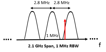
Input signals may fall in between two adjacent filter curves or into the shoulder of a filter curve. Consequently, the signal will be attenuated and the analyzer display would show a lower amplitude value – the measurement value would be incorrect. The displayed frequency will be corresponding with the center frequency of the closest measurement frequency point and the offset would be incorrect as well.
Let´s take another example and look at a typical conducted emission measurement. In most cases, this measurement covers the frequency range up to 30 MHz and requires a CISPR RBW of 9 kHz. Attempting to make a full sweep across the entire 30 MHz results in a spacing of 30 MHz / 751 = 39.9 kHz. A significant part of the spectrum would not be measured at all:
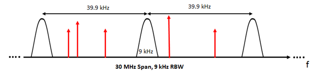
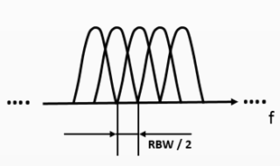
In order to cover the entire spectrum within the span of a frequency sweep, CISPR 16 specifies that adjacent frequency points shall not be spaced more than half of the resolution bandwidth. In the case of the example above, the spacing shall not be more than 9 kHz / 2 = 4.5 kHz.
With this information in mind, the frequency span settings have to be chosen in order to fulfill the frequency spacing and RBW specifications of CISPR 16:
| Number of measurement points per sweep: 751 (Siglent SSA3021X) | ||
| Frequency range | CISPR filter bandwidth | Maximum frequency span |
| 9 kHz – 150 kHz | 200 Hz | 75 kHz |
| 150 kHz – 30 MHz | 9 kHz | 3.38 MHz |
| 30 MHz – 1 GHz | 120 kHz | 45 MHz |
| Above 1 GHz | 1 MHz | 375 MHz |
Consequently, a conducted emission measurement for the frequency range 150 kHz to 30 MHz has to be split into at least 29.85/3.38 = 9 segments with a span of 3.38 MHz.
Doing such a measurement manually would be a tedious process. Various analyzers let you increase the default number of measurement points to a higher value. Newer analyzers also offer the capability to select standard conformant EMI measurement routines, which also ensure that adjacent measurement points have the correct frequency spacing. The disadvantage is that the resulting graph is still limited to the number of available display pixels.
Tekbox offers EMCview EMI measurement software, which splits the measurement into consecutive sweep segments. The measurement values of all sweeps are then stitched together to a single graph for easy analysis and reporting. EMCview also simplifies EMI measurements by providing a vast list of pre-configured measurements.
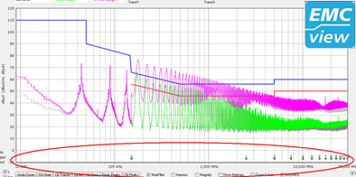
Figure 3: Conducted noise measurement with EMCview. The 30 MHz sweep is built from 12 segments with a 2.5 MHz span each.
3.4 Sweep time
CISPR 16 differs between wideband and narrowband noise. Narrowband noise is typically caused by clock signals. Wideband noise is caused by data signals. As the spectrum of data signals is caused by a more or less arbitrary bit sequence, it is dynamic and wideband. Furthermore, signals may be present or not, depending on tasks running on the controller. Sweeping too fast would miss pulses and not correctly measure the wideband noise spectrum.
Consequently, CISPR 16 specifies minimum sweep times, depending on frequency range and detector:
| Frequency range | Peak detector | Quasi-peak detector |
| 9 kHz – 150 kHz | 100 ms / kHz | 20 s / kHz |
| 150 kHz – 30 MHz | 100 ms / MHz | 200 s / MHz |
| 30 MHz – 1 GHz | 1 ms / MHz | 20 s / MHz |
Table 2: CISPR 16 minimum sweep times for specific frequency ranges.
CISPR 25 specifies minimum sweep times below:
| Frequency range | Peak detector | Peak detector | Quasi-peak detector |
| 150 kHz – 30 MHz | 10 s / MHz | 10 s / MHz | 200 s / MHz |
| 30 MHz – 1 GHz | 100 ms / MHz | 100 ms / MHz | 20 s / MHz |
| above 1 GHz | 100 ms / MHz | 100 ms / MHz | n.a. |
Table 3: CISPR 16 minimum sweep times for specific frequency ranges.
Longer sweep times have an averaging effect, reducing the noise level:
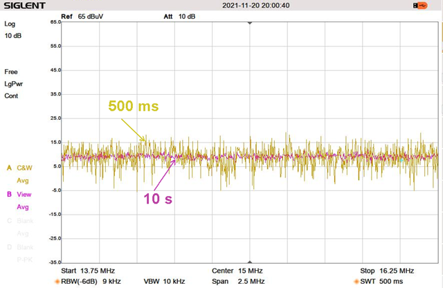
Figure 4: Analyzer DANL with 500 ms sweep time versus 10 s sweep time.
3.5 Detectors
Most conducted and radiated emission tests have limits specified for average detector and quasi-peak detector.
Whereas measurement scans with average and peak detectors can be carried out reasonably quickly, quasi-peak detectors require a measurement time of 1 second per measurement point for measurement receivers and a similarly long time for spectrum analyzers. A single, complete measurement scan may take several hours when carried out with quasi-peak detectors.
However, there is a workaround, which reduces measurement time significantly:
The measurement result of the peak detector is always higher than the measurement result of the average detector.
The measurement result of the quasi-peak detector will always be somewhere in between the results of the average and positive peak detector. The measurement result of the quasi-peak detector will never be higher than the measurement result of the positive peak detector.
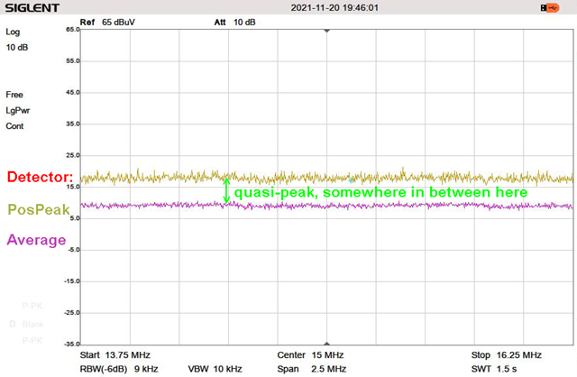
Figure 5: Example of the differences between the positive peak and average detector types.
Consequently, a complete scan will be carried out, using the peak detector and the result will be compared against the quasi-peak limits. If the peak detector measurement is within QP limits, the EUT has passed the test. If the peak detector result has a few spurious peaks, which cross the limit line, there is still the chance that the quasi-peak result is within the limits. However, if the spurious peaks are 10 dB or more above limits, the chance is pretty slim.
To verify, a selective re-measurement, using the quasi-peak detector, will be carried out at only the frequency points where the peak detector measurement crosses the limit line.
When selectively re-measuring spurious peaks with critical amplitudes, it also needs to be considered that the spurious peaks may have drifted in frequency in the time that passed between peak detector measurement and selective re-measurement with the quasi-peak detector. Peaks originating from switched-mode regulators may drift considerably over time and temperature. Doing a selective re-measurement may completely miss the spurs at a later time or have the spur frequency offset far enough to obtain a wrong measurement result. EMCview offers a selective measurement option considering frequency drift. Instead of just measuring at a single frequency, the quasi-peak measurement can be carried out across several adjacent frequency points. EMCview will then make a peak search through these frequency points to ensure capturing the correct quasi-peak amplitude.
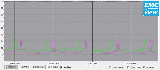
Figure 6: Example of spurious drifting over time. Both measurements were taken with the same settings, but with a time difference of 15 minutes.
The screenshot below shows a plot from a test house showing the concept of selective quasi-peak measurement. The orange graph shows the peak detector measurement with the blue markers at the frequencies, where the quasi-peak limits are violated. The red markers show the results of selectively re-measuring with the quasi-peak detector.
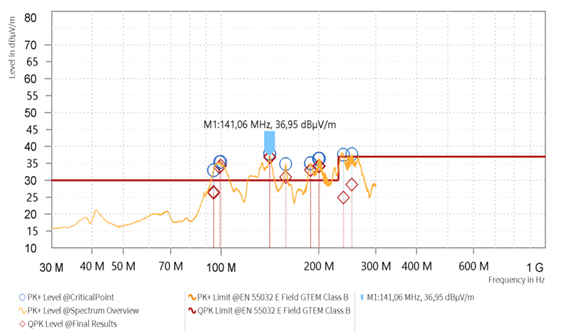
Figure 7: Example of a test house report showing selective QP scan.
4. Internal attenuator, pre-amplifier
When setting up the spectrum analyzer for any EMC measurement, careful choice of internal attenuator settings is essential.
The screenshot below shows the effect of the internal attenuator and pre-amplifier settings on the DANL of the spectrum analyzer.
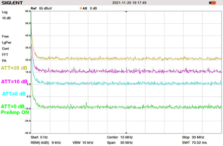
Figure 8: DANL versus internal attenuator / pre-amplifier settings. RF input terminated with 50 Ohm.
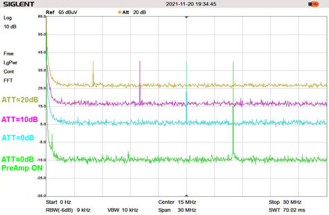
Figure 9: Power versus internal attenuator/pre-amplifier settings. RF input fed with CW signal; constant amplitude but shifted 5 MHz at each setting for better visibility.
When performing conducted emission testing, there is a high probability for high amplitude spurs. Choosing 0 dB attenuation and eventually turning on the pre-amplifier at the same time may cause intermodulation distortions and/or ADC saturation. Consequently, the default settings for most conducted emission tests in EMCview are 20 dB internal attenuation and pre-amplifier off. Some standards, however, such as CISPR 25 Class 5 conducted emissions, voltage method, have very low limit levels and require less internal attenuation.
Radiated emission measurements require very high sensitivity. Corresponding default EMCview project settings are typically 0 dB internal attenuation and pre-amplifier on.
CISPR 16 specifies that the base noise of the measurement setup has to be at least 6 dB below the limit lines in order to have sufficient dynamic range to reliably measure critical spurious.
5. Distortion considerations
The spectrum analyzer itself may produce distortion products, and potentially disturb measurements, if strong signals are applied to the RF input. As spectrum analyzers contain components with non-linear behavior such as mixers and amplifiers, they will always generate some distortion products. This internal distortion can, at worst, completely cover up the distortions created by the Equipment Under Test (EUT).
The user needs to understand how distortion is related to the input signal, to determine for a particular measurement, whether or not the distortion caused by the analyzer, will affect the measurement.
The dominant non-linear distortions are second-order and third-order harmonics.
The second-order distortion increases as a square of the amplitude of the fundamental signal, and the third-order distortion increases as a cube.
When the fundamental power is in/decreased 1 dB, the second-order distortion in/decreases by 2 dB.
When the fundamental power is in/decreased 1 dB, the third-order distortion in/decreases 3 dB.
Using attenuators, it can be determined whether any spurious come from the signal source or whether they are generated by the spectrum analyzer.
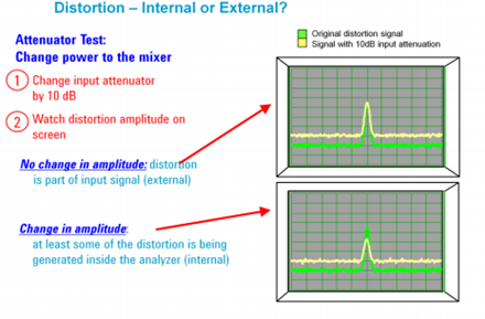
Figure 9: A technique to determine the source of distortion.
6. General sensitivity considerations
6.1 Conducted noise testing with LISN
When choosing the amplitude settings of the spectrum analyzer, compare the limit lines against the DANL of the analyzer. Figure 10 below shows that there is 80 dB of dynamic range between limit lines and DANL if the analyzer will be set to maximum sensitivity. On the other hand, CISPR 16 requires a minimum spacing of 6 dB between DANL and limit lines.
The analyzer settings should be modified to Att = 20 dB and PreAmp = OFF. This would raise the noise floor approximately 40 dB, but still leave 40 dB of dynamic range below the limit lines. The sensitivity is still more than sufficient and the risk of creating non-linear distortions or ADC saturation is significantly reduced.
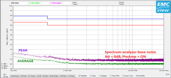
Figure 10: Example CISPR 32 Class A, conducted emissions, mains supply line.
Whenever choosing the analyzer settings, first have a look at the limit lines and then decide on the amplitude settings.
Most standards have the limits for conducted noise settings sufficiently high, to operate with at least 20 dB attenuation and without a pre-amplifier.
Exceptions are automotive standards such as CISPR 25 Class 5 or generic car manufacturer standards, which require higher sensitivity:
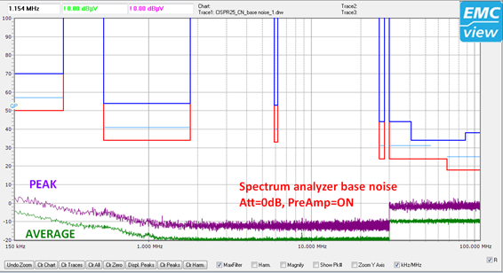
Figure 11: Example of CISPR 25 Class 5 conducted base noise level sweep.
In case of nonlinear distortion issues, the pre-amplifier could be turned off at the most, in order to leave sufficient dynamic range for the frequency range above 60 MHz.
6.2 Conducted noise testing with RF current probes
When performing conducted noise measurements with RF current monitoring probes, the trans-impedance value in dBΩ subtracted from the measurement value in dBµV gives the RF current in dBµA.
dBµA = dBµV – dB(Ω)
In the case of an RF current monitoring probe with a trans-impedance of 0 dBΩ, the readings at the probe output in dBµV are equivalent to the RF current passing the probe cross-section in dBµA.
Figure 12 below shows the limits for a CISPR 25 Class 5 Current Method measurement. Note that the limits are given in dBµA.
The displayed trace corresponds to settings for maximum analyzer sensitivity: Att = 0dB, PreAmp = ON
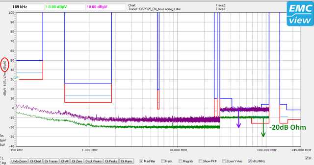
Figure 12: Example of CISPR 25 Class 5 Current Method.
If an RF current probe with a trans-impedance of 0 dBΩ would be used for this measurement, the base noise would collide with the limits above 25 MHz, even at maximum sensitivity settings.
In order to carry out a useful measurement, an RF current monitoring probe with a trans-impedance of at least 15 dBΩ to 20 dBΩ is required.
Figure 13 below shows the base noise of a CISPR 25 class 5 Current Method measurement, using a TBCP2-500 RF current monitoring probe from Tekbox with the spectrum analyzer internal attenuation set to 0 dB and the pre-amplifier turned on. This setup gives sufficient dynamic range to carry out a useful measurement:
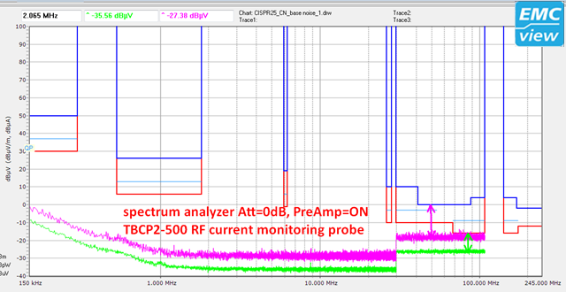
Figure 13: Example of CISPR 25 Class 5 Current Method with a Tekbox TBCP2-500 RF probe.
6.3 Radiated noise testing with TEM-cells
Transverse-Electromagnetic Cells (TEM Cells) are a stripline device for radiated emissions and immunity testing of electronic devices.
Radiated noise testing in TEM cells can be started with the analyzer sensitivity set to maximum. There is typically no big risk of overdriving or damaging the analyzer. In case of high amplitude emissions, the settings can be adjusted accordingly.
Figure 14 below shows the limits for CISPR 25 Class 5 TEM Cell versus spectrum analyzer base noise with the spectrum analyzer internal attenuation set to 0 dB and the pre-amplifier turned on
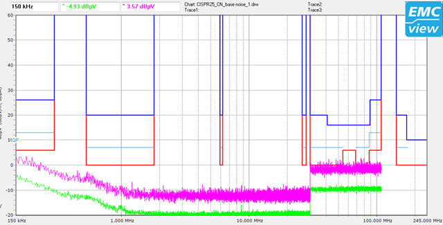
Figure 14: CISPR 25 Class 5 TEM example
6.4 Radiated noise testing with antennas
Radiated noise limits are given in dBV/m in most cases. In order to convert the measurement result from Voltage at 50 Ohm [dBµV] to field strength [dBµV/m], it is necessary to know the antenna characteristics versus frequency. Measurement antennas always come with an antenna factor table. The antenna factor needs to be added to the voltage displayed at the analyzer in order to obtain the field strength:
dBµV/m = dBµV + AF
Consequently, the antenna factor also adds to the base noise and reduces the dynamic range of the measurement.
EMC measurement antennas have typically a large bandwidth. The larger the bandwidth, the lower the gain and the higher the antenna factor.
Figure 15 below shows CISPR32 Class A radiated emission limits in dBµV/m for a measurement distance of 3 m.
The dark green graph shows the spectrum analyzer base noise in dBµV with the internal attenuation set to 0 dB and the pre-amplifier turned on.
The light blue graph shows the base noise in dBµV/m when used together with the 30 MHz – 1GHz TBMA1 biconical antenna from Tekbox.
The dark blue graph shows the base noise in dBµV/m when used together with the 30 MHz – 300MHz TBMA2 biconical antenna from Tekbox.
The light green graph shows the base noise in dBµV/m when used together with the 250 MHz – 1.3 GHz TBMA3 logarithmic periodic antenna from Tekbox.
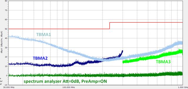 Figure 15: CISPR32 Class A radiated emissions for various antennas
Based on the above analysis of the base noise, there seems to be sufficient dynamic range for carrying out CISPR 32 Class A radiated noise measurements using the Siglent SSA3021X spectrum analyzer and any of the mentioned EMC measurement antennas from Tekbox.
However, the above graphs would only be realistic when carrying out the measurement in a shielded anechoic chamber. In reality, EMC pre-compliance radiated emission tests are often carried out in a non-shielded environment such as a development laboratory or an industrial site.
Figure 16 shows the output of the TBMA1 measurement antenna, in an industrial environment.
In the frequency range from 30 MHz to 100 MHz, the ambient noise already exceeds the CISPR 32 Class A radiated limits and severely handicaps the radiated noise measurement of any EUT. Even at higher frequencies, it will become very difficult to differentiate between ambient noise and noise originating from the EUT:
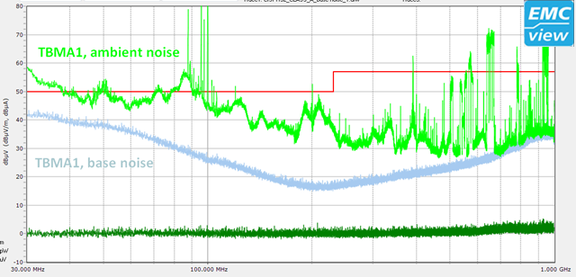 Figure 16: Example of ambient scan in an industrial environment
However, there are a few solutions to combat the ambient noise issue. Try to find a location with less ambient noise. A flat roof or a test site in a field are often less noisy than an industrial site. When measuring inside a lab, turn off all equipment nearby to eliminate noise from switched-mode power supplies.
Move the antenna closer to the EUT. Reducing the measurement distance from 3 m to 1 m is equivalent to approximately 10 dB less free space loss or lifting the limits 10 dB higher. However, consider that the antenna may move into the near field zone at lower frequencies.
Use a lower bandwidth measurement antenna with lower antenna factors.
Measure your EUT inside a TEM cell to get a plot of the critical emissions. Knowing the frequencies of critical spurious, repeat the antenna measurement, but reduce span and RBW. Zoom in on critical frequencies, so to say.
Carry out the measurement at night, when there is typically less ambient noise.
7. Input protection
Whenever working with spectrum analyzers, be aware that excessive input power, voltage transients or ESD can destroy the RF-frontend. Spectrum analyzers typically have a maximum CW input rating in the range of +20 dBm to +30 dBm. Unlike oscilloscopes, spectrum analyzer inputs are not protected or only vaguely protected. A simplified RF frontend is shown below:
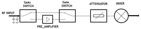
The diodes at the input typically serve as ESD protection diodes. In order to fully protect the input with a limiter, shunt diodes would need to be combined with a series resistor to limit forward current in case of excessive input signal power. Consequently, a classic current limiting resistor solution cannot be implemented, as it would increase the input impedance of the analyzer.
A limiter could be implemented by combining it with an attenuator however, this would degrade the sensitivity of the analyzer and limit its use.
The first weak link of the input chain is the RF switch. Typical EMI spectrum analyzers use integrated GaAs switches. GaAs switches are inherently weak at low frequencies. Many GaAs switches are not even specified with respect to maximum input power at low frequencies, down to 9 kHz.
Below is an example of an “honest” data sheet of a typical GaAs switch:
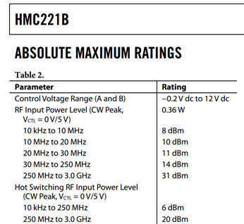
The maximum RF input power ratings versus frequency clearly show the degradation at low frequencies.
When carrying out conducted noise tests of switched-mode power supplies, the highest spurious levels occur at relatively low frequencies. Sub-harmonics are even more critical. These are typically at frequencies significantly below 100 kHz and often go completely unnoticed, as most tests start at 150 kHz. You may carry out a conducted noise test and wonder, why the analyzer beeps and displays an ADC overflow warning, despite all spurious being well below limits. What drives the attenuator into saturation may be a very high amplitude sub-harmonic at 6 kHz.
In case that you notice that your signals are in the range of 20 dB lower than what they actually are, disaster already happened. The first GaAs switch is already damaged. In most cases, it fails with a short on the RF path and protects the following components, but in extreme cases, the damage will reach as far as the first mixer.
In order to prevent such things happen, you always should start investigating any new EUT using external attenuators or a combined attenuator/limiter, both also available from Tekbox. With an external 20 dB attenuator or limiter attached to the analyzer input, have a look at the spectrum at very low frequencies and ensure that there are no signals with critically high amplitude.
Alternatively, you can first connect an oscilloscope to the LISN RF output and check the EUT emissions in the time domain. In order to establish the same impedance level as with a connected spectrum analyzer, terminate the oscilloscope input with a 50 Ohm feedthrough or switch the input to 50 Ohm, if the scope offers this feature.
Here are some guidelines when performing conducted emission measurements with a LISN:
- Leave the RF output of the LISN unconnected
- Connect the EUT to the LISN
- Connect the LISN to the isolation transformer
- Power on the EUT
- Check the RF output of the LISN using a scope and/or the analyzer with an external 20 dB attenuator or combined attenuator/limiter
- Connect the RF cable from LISN output to the spectrum analyzer input
- Carry out the conducted noise scan
- Disconnect the RF cable
- Power off the EUT
NOTE: The purpose of having the analyzer disconnected during power cycling (ON/OFF) the EUT is to avoid voltage transients due to back EMF, especially of highly inductive loads such as motors or switched-mode power supplies. These signals can easily be large and fast enough to cause permanent damage to the sensitive RF front end of the analyzer.
In cases where the EUT produces subharmonics, place a suitable highpass filter at the RF input of the spectrum analyzer. The Tekbox TBFL1 transient limiter not only contains a combined attenuator/limiter, but also a 9 kHz highpass filter. If the subharmonic frequency is above 9 kHz, connect a 150 kHz highpass.
8. History
| Version | Date | Author | Changes |
| V 1.0 | 22.11.2021 | Mayerhofer | Creation of the document (Tekbox) |
| V.1. | 03.12.2021 | Chonko | Grammar, typos, and re-arranged sections for clarity |